On a previous video/blog post, I talked about production planning using an example of selling art on the beach. One simplification of that model was the assumption that everything that we build can be sold.

You can check the pluto notebook html or download the notebook.
I have an excert down here, but for more details, check the video.
If you just want, you can just skip to questions.
As we saw on last episode, Javier is creating and selling his art on the beach. However, we assumed that everything that Javier builds will be sold, which is unrealistic.
Now, we have to deal with a more realistic scenario, in which the demand for Javier’s product is not infinite. We will still need assumptions, but the model is a bit more realistic.
Strategy 1: Sell excess inventory at a discount
The first strategy is simple. If there is no more demand for the products, Javier sells them at a discounted price.
For that, we need to assume that
- Javier knows the demand for each of their products under the price that he decided to sell them;
- Javier discounted price is low enough to sell all of the remaining products.
Modeling
Our new model is pretty much the same as before, but I will bring the new parts to your attention.
How to model discounted price
(see also piece-wise concave linear objective)
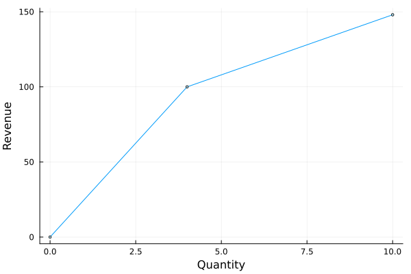
Let’s consider only the bracelet: selling price €25 up to 4 units and €8 after that.
One way of describing our objective is by defining the nonlinear function $\text{revenue}(q)$:
$$\text{revenue}(q) = \left\{\begin{array}{cc} 25q, & 0 \leq q \leq 4, \\ 25\times 4 + (q - 4)\times 8, & q > 4. \end{array}\right.$$
This is not linear, though, so to maximize this function we need to some modeling magic, and in this case there is a very simple approach.
First, we split the quantity decision variable $q$ into two parts:
- Quantity under demand: $\underline{q}$
- Quantity over demand: $\overline{q}$
Then, the revenue function can be expressed as
$$25\underline{q} + 8\overline{q} \quad \text{subject to} \quad \underline{q} \leq 4, \ \overline{q} \geq 0$$
And whenever cost is not important, use $\underline{q} + \overline{q}$ instead of $q$. We can, to improve readability, create that as an expression $q = \underline{q} + \overline{q}$.
It might not be clear at first why this works, since $q = \underline{q} + \overline{q}$ does not imply that we are selling first the normal priced items. The reason that it works is that we are maximizing the revenue. This means that if you have to write $7 = \underline{q} + \overline{q}$ to maximize revenue, one would prefer $\underline{q} = 4$ and $\overline{q} = 3$.
The animation below shows the function on two variables and the best choice given a production.
Notice that the new constraints $\underline{q} \leq 4$ and $\overline{q} \geq 0$ are necessary.
Model
Sets:
- Products: $p \in \mathcal{P}$
- Materials: $m \in \mathcal{M}$
Parameters:
| Name | Unit | Identifier | Set |
|---|---|---|---|
| Time availability | h | $\text{time_available}$ | |
| Selling price of $p$ | € / unit | $\text{selling_price}_p$ | $p \in \mathcal{P}$ |
| (New) Discounted price of $p$ | € / unit | $\text{discounted_selling_price}_p$ | $p \in \mathcal{P}$ |
| (New) Demand for product $p$ | unit | $\text{demand}_p$ | $p \in \mathcal{P}$ |
| Hours to assemble product $p$ | $h$ / unit | $\text{assemble_time}_{p}$ | $p \in \mathcal{P}$ |
| Material $m$ cost | € / [$m$] | $\text{material_cost}_m$ | $m \in \mathcal{M}$ |
| Amount of $m$ per unit of $p$ | [$m$] / unit | $\text{mat_per_prod}_{p,m}$ | $p \in \mathcal{P}, m \in \mathcal{M}$ |
Variables:
As mentioned, the production variable is split into two parts, one to possibly satisfy the demand, and one for extra products sold.
- Amount of product $p$ assembled and sold at full price (unit): $\text{prod_normal}_p, \quad p \in \mathcal{P}$
- Amount of product $p$ assembled and sold at discount (unit): $\text{prod_extra}_{p}, \quad p \in \mathcal{P}$
Expressions:
As mentioned before, let’s create a helper expression for the total amount of products produced. This essentially allows us to reuse all other expressions and constraints.
- Amount produced and sold of product $p$: $$\displaystyle \text{prod}_p = \text{prod_normal}_{p} + \text{prod_extra}_{p}, \quad p \in \mathcal{P}$$
The revenue also changes to differentiate the products:
- Revenue: $$\text{revenue} = \sum_{p \in \mathcal{P}} \bigg( \text{selling_price}_p \times \text{prod_normal}_{p} + \text{discounted_selling_price}_p \times \text{prod_extra}_{p} \bigg)$$
The other expressions are the same as before.
Objective:
The objective hasn’t changed.
- Maximize profit: $\text{maximize} \quad \text{revenue} - \text{total_material_cost}$
Constraints:
Now, to finalize, we have the extra constraints mentioned before.
Production under demand: $\text{prod_normal}_{p} \leq \text{demand}_p, \quad p \in \mathcal{P}$
Nonnegativity: $\text{prod_normal}_{p}, \ \text{prod_extra}_{p} \geq 0$
Integer production: $\text{prod_normal}_{p}, \ \text{prod_extra}_{p} \in \mathbb{Z}$
Time Availability: $\text{spent_time} \leq \text{time_available}$
Results
The solution is below. Check the video for the implementation details.
Strategy 2: Demand is a function of price
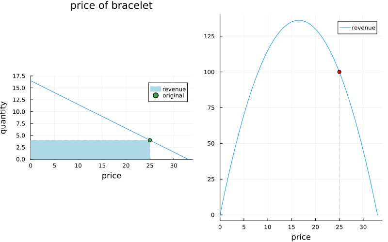
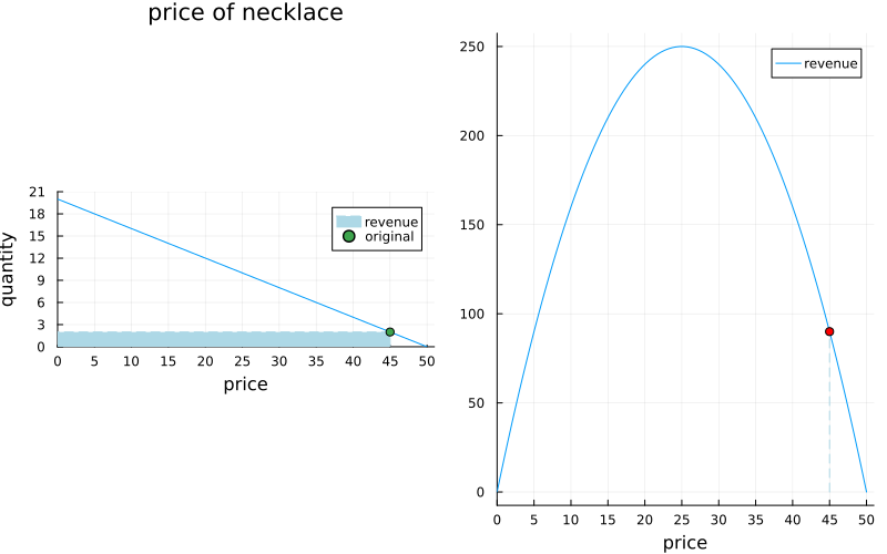
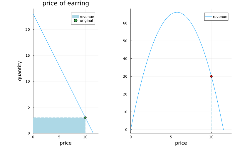
Our second approach is to consider that the demand for the products depends on their price and to add this relation into the model. In other words, we are not only deciding how many products we will build, we will decide at which price we will sell them.
To do that we have to assume that we know how the demand depends on the price, which is not something trivial to figure out. For today, let’s assume that this dependency will be linear:
$\text{demand} = \text{intercept} + \text{slope} \times \text{price},$
and that we now the intercept and slope values for each product.
Below are the plots of the values that we assume represent the demand.
Modeling
There are a few more nuanced differences in this model.
Sets:
- Products: $p \in \mathcal{P}$
- Materials: $m \in \mathcal{M}$
Parameters:
| Name | Unit | Identifier | Set |
|---|---|---|---|
| Time availability | h | $\text{time_available}$ | |
| (new) Demand of product $p$ (intercept) | unit | $\text{demand_intercept}_p$ | $p \in \mathcal{P}$ |
| (new) Demand of product $p$ (slope) | unit / [€] | $\text{demand_slope}_p$ | $p \in \mathcal{P}$ |
| Hours to assemble product $p$ | h / unit | $\text{assemble_time}_p$ | $p \in \mathcal{P}$ |
| Material $m$ cost | € / [$m$] | $\text{material_cost}_m$ | $m \in \mathcal{M}$ |
| Amount of $m$ per unit of $p$ | [$m$] / unit | $\text{mat_per_prod}_{p,m}$ | $p \in \mathcal{P}, m \in \mathcal{M}$ |
Variables:
The selling price is not a parameter anymore.
Instead, we have a variable, which we called decided_price to differentiate, that will inform the value at which the product is sold.
- Amount of product $p$ assembled and sold (unit): $\quad \text{prod}_p, \quad p \in \mathcal{P}$
- (New) Price of product $p$ (€): $\quad \text{decided_price}_p, \quad p \in \mathcal{P}$
Expressions:
A few things changed here. First, the demand is an expression now, which we will use in the constraints.
Second, and maybe most important, the revenue is quadratic now. This by itself is not an issue, but when coupled with the integrality of the variable $\text{prod}_p$, we have a much harder problem on our hands.
(New) Demand: $$\begin{align}\text{demand_given_price}_p = & \text{demand_intercept}_p + \\ & \text{demand_slope}_p \times \text{decided_price}_p, \quad p \in \mathcal{P} \end{align}$$
Revenue: $\displaystyle \text{revenue} = \sum_{p \in \mathcal{P}} \text{decided_price}_p \times \text{prod}_p$
The other expressions have not changed.
Objective:
- Maximize profit: $\text{maximize} \quad \text{revenue} - \text{total_material_cost}$
Constraints:
The new constraint of the model is relating the production to the price via the demand. Notice that the actual constraint could be written using equality. However, since the production is an integer, and the price is a floating-point number, it might be that the actual demand value (which should be an integer), is just a little bit off. Depending on the solver, it might help.
- (New) Produce what you can sell: $$\text{prod}_p \leq \text{demand_given_price}_p, \quad p \in \mathcal{P}$$
- Time Availability: $\text{spent_time} \leq \text{time_available}$
- Non-negativity: $\text{prod}_p, \ \text{decided_price}_p \geq 0, \quad p \in \mathcal{P}$
- Integer production: $\text{prod}_p \in \mathbb{Z}$
Implementation
Last time we used the Cbc solver to solve our problem. It had integer variables, but it was otherwise linear.
This time, the objective is quadratic. Therefore, we need to use a different solver. SCIP is a good open-source choice.
Results
The solution is below. Check the video for the implementation details.
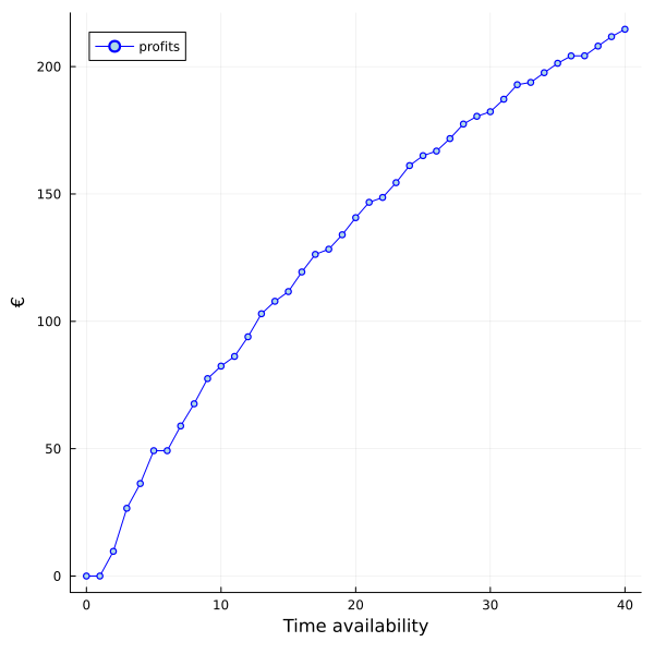
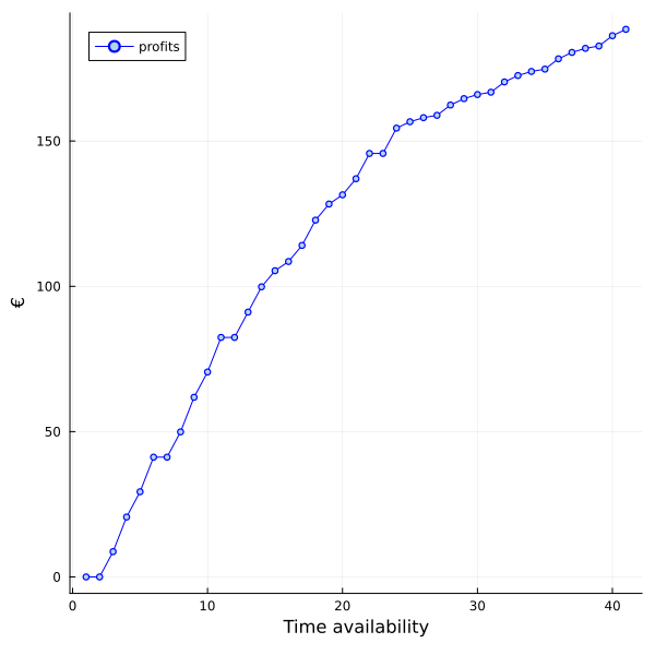
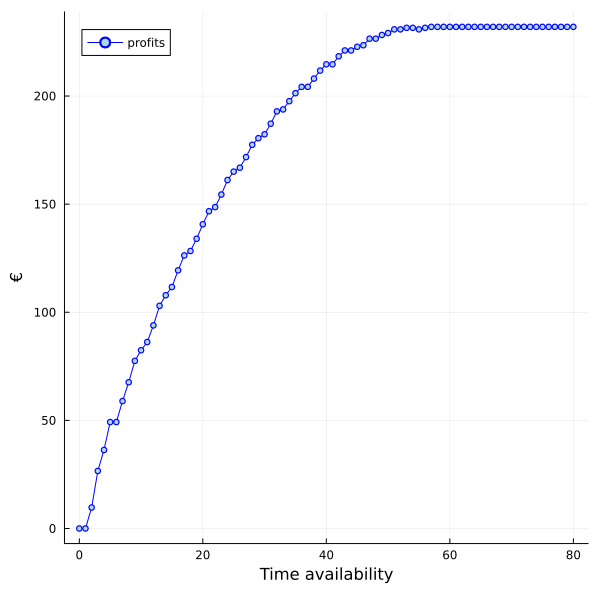
Notice that there are diminishing returns in producing more. Furthermore, if you decrease the price too much to sell more products, you start to lose money. Therefore, eventually you stop producing more, and your profit stabilizes. The plot below shows the situation if you worked more than 40 hours:
Questions
- In strategy 1, what if you had extra levels of price? For instance, for new products, you produce few with a high price. After selling those, you have a secondary price for a larger amount of products. After that, you have a sale for the remaining products. How do you model that?
- In strategy 2, the profit stabilizes after working about 60 hours. If, for instance, Javier gets a partner, it wouldn’t make sense to work more than 30 hours each to satisfy the demand. What would you do in this situation?